
This chapter talks about how to represent curves mathematically in 3D. Recreating a curve from its mathematical definition is relatively easy; the tricky part is obtaining a curve with desired properties, or alternatively, making a tool that designers can use to draw such curves. Our goal in this chapter is to provide a graceful and intuitive introduction to the mathematics of curves. In comparison with most of the other books on the subject, our aim is to hit the most important points, without stopping every other paragraph to prove that what we are saying is true. (We will, however, stop periodically to discuss correct pronunciation, which is probably appropriate considering that most of the people who developed the math we'll be using in this chapter were French.) Curves and splines are very useful for all sorts of reasons. There are obvious applications such as moving objects around on curved trajectories. But then the coordinates of our curve need not have a spatial interpretation; essentially, any time we wish to fit a function for a color, intensity, or other property to given data points, we have a potential application for curves and splines.
The chapter is divided roughly into two parts. The first part is about simple, “short” curves that can be described by one equation.
- Section 13.1 introduces the specific type of curve we focus on almost exclusively: the parametric polynomial curve. (It pays special attention to cubic polynomials.)
- Section 13.2 describes polynomial interpolation, whereby a curve is threaded through specified control points.
- Section 13.3 discusses Hermite form, which describes a curve in terms of its endpoints and the derivatives at those endpoints.
- Section 13.4 shows how the Bézier form specifies the curve endpoints, plus interior control points that influence the shape of the curve but are not interpolated.
- Section 13.5 shows how to subdivide a curve into smaller pieces.
The second half of the chapter covers splines, which are longer curves created by joining together multiple curves in succession.
- Section 13.6 introduces some basic notation, terminology, and concepts.
- Section 13.7 discusses how to join together Hermite or Bézier curves into a spline.
- Section 13.8 considers continuity (smoothness) conditions for splines.
- Section 13.9 ends the discussion on splines by considering various methods for automatically determining the tangents of a spline at the control points.
13.1Parametric Polynomial Curves
We focus here almost exclusively on one particular type of curve, the parametric polynomial curve. It's important to understand what the two adjectives parametric and polynomial mean, so Section 13.1.1 and Section 13.1.2. discuss them in detail. Section 13.1.3 reviews some useful alternate notation. Section 13.1.4 examines the straight line, which is a particularly instructive example of a parametric polynomial curve. Section 13.1.5 considers the relationship between the endpoints of the curve and polynomial coefficients. Section 13.1.6 discusses derivatives, such as velocity and acceleration, and shows how they are related to tangent vectors and local curvature.
13.1.1Parametric Curves
The word parametric in the phrase “parametric polynomial curve”
means (not altogether surprisingly) that the curve can be described by a function of an
independent parameter, which is often assigned the symbol
We briefly introduced parametric representation of geometric primitives in
Section 9.1. Let's take a moment to review some of the
alternative forms from that section so we can understand ways of describing a curve that are
not parametric. An
implicit representation is a relation that is true for all points in the shape being
described; for example, the unit circle can be described implicitly as the set of points
satisfying
The curve
Sometimes we think of the position function
13.1.2Polynomial Curves
Now that we know what the adjective parametric means, let's turn our attention to the
second important word, polynomial. A polynomial parametric curve is a parametric curve
function
The number
We've already seen an example of a curve function that is parametric but not polynomial—the
parametric circle given by Equation (13.1). The expressions for
Of most interest to us are the parametric polynomial curves of degree 3, known as cubic curves. Cubic curves are those that can be expressed in the form shown in Equation (13.2).
This method of describing curves is often called the monomial form or the power
form, to emphasize the fact that the curve is specified by listing the coefficients of the powers
of
Once we have the coefficients, it's easy to reconstruct the curve
by evaluating the function
Suppose we need to render a curve. One simple way to do this is to approximate it with, say, 10
line segments, sampling the curve at
But where do the coefficients
13.1.3Matrix Notation
We can rewrite the monomial form (Equation (13.2)) in
several different ways. It's useful to be able to refer to a coefficient for a particular
coordinate. For example, in 2D let's use the notation
Some books are fond of writing this more compactly by using matrix notation. Let's put the
coefficients into a matrix
Now we can express our curve function
The matrix
When dealing with a higher degree polynomial, the matrix
13.1.4Two Trivial Types of Curves
Although you're reading this section because you want to learn how to draw a curve, allow a brief digression to mention two trivial types of “curves”: a straight line segment and a point.
We showed how to represent a line segment parametrically in
Section 9.2 when we discussed rays. Consider a ray from the point
Observe that this is a polynomial of the type we've been considering,
where
As boring as lines are, there's an even less interesting shape that can be represented in
parametric polynomial form: the point. Lowering the degree of the polynomial from 1 to 0 results
in a so-called
constant curve. In this case, the function
13.1.5Endpoints in Monomial Form
Clearly, one of the most basic properties of a curve that we want to control are the locations of
its start and end,
In other words,
So the endpoint of the curve is given by the sum of the coefficients.
13.1.6Velocities and Tangents
We can think of curves as being either static or dynamic. In the static sense, a curve defines a
shape. We operate in this mode of thinking when we use a curve to describe the cross section of
an airplane wing or a portion of the letter “S” in the Times Roman font. In the dynamic sense,
a curve can be a trajectory or path of an object over time, with the parameter
If we consider only the static shape of the curve, then the timing of the curve doesn't matter and our task is a bit easier. For example, when defining a shape, it doesn't matter which endpoint is considered the “start” and which is the ”end”; but if we are using the curve to define a path traversed over time, then it matters very much where the path starts and where it ends.
Using the dynamic mental framework and thinking about curves as paths and not just shapes, some
natural questions to ask are, “In what direction is the particle moving at a given point in
time?” “How fast is it moving?” These questions can be answered if we create another function
The phrase “instantaneous velocity” implies that the velocity changes over time. So the next
logical step is to ask, “How fast is the velocity changing?” Thus it is also helpful to define
an instantaneous acceleration function
If you've had at least a semester of calculus, or if you read Chapter 11,
you should recognize that the velocity function
We're considering curves where
The derivatives of cubic curves are especially notable and appear several times in this chapter.
Now let's examine velocity and acceleration in the special case of a parametric ray. Applying the velocity and acceleration functions of Equations (13.5) and (13.6) to the original parameterization of a ray from Equation (13.3) yields
Velocity and acceleration of a rayAs we'd expect, the velocity is constant; there is no acceleration.
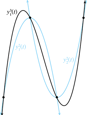
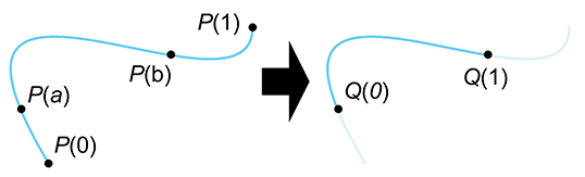
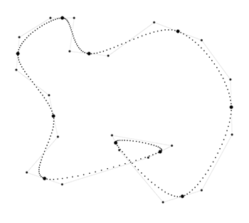
Sometimes two curves define the same shape but different paths (see
Figure 13.1). We've already mentioned one example of this: if we
traverse the path backwards it still traces out the same shape. A more general way to generate
alternate paths that trace out the same shape is to reparameterize the curve. For example,
let's reparameterize our line segment
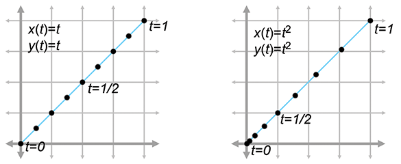
Notice that both curves in Figure 13.1 define the same static shape, but different paths. On the left, the particle moves with constant velocity, but on the right it starts out slowly and accelerates to the finish.
If we are using a curve as a shape and not a path, then this reparameterization doesn't have a visible effect. But that doesn't mean that the derivatives of the curve are irrelevant in the context of shape design. Imagine that we are creating a font using a curve to define a segment of the letter S. In this instance, we might not care about the velocity at any point, but we would care very much about the tangent of the line at any given point. The tangent at a point is the direction the curve is moving at that point, the line that just touches the curve. The tangent is basically the normalized velocity of the curve. Let's formally define the tangent of a curve to be the unit vector pointing in the same direction as the velocity:
The tangent vectorHigher derivatives also have geometric meaning. The second derivative is related to
curvature, which is sometimes denoted
13.2Polynomial Interpolation
You are probably already familiar with linear interpolation. Given two “endpoint” values, create a function that transitions at a constant rate (spatially, in a straight line) from one to the other. We say that the function interpolates the two control points, meaning that it passes through the control points and can be used to compute intermediate values.
Polynomial interpolation is similar. Given a series of control points, our goal is to construct
a polynomial that interpolates them. The degree of the polynomial depends on the number of
control points. A polynomial of degree
In the context of curve design, to say that a curve interpolates control points is to place specific emphasis on the fact that the curve passes through the control points. This is to be contrasted with a curve that merely approximates the control points, meaning it doesn't pass through thepoints but is attracted to them in some way. We use the word“knot” to refer to control points that are interpolated, invoking the meta-phor of a rope with knots in it. It would seem at first glance that the availability of an interpolation scheme would make any approximation schemeobsolete, but we'll see that approximation techniques do have their advantages.
Polynomial interpolation is a classic problem with several well-studied solutions. Since this is a book on 3D math we cast the discussion primarily in geometric terms, but be aware that most of the literature on polynomial interpolation adopts a more general view, because the task of fitting a function to a set of data points has broad applicability.
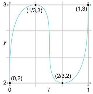
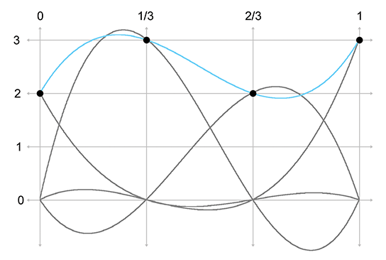
To facilitate the discussion we use a particular example curve, shown in
Figure 13.2. It's somewhat like an S turned on its
side. We've marked the four control points on the curve that we are attempting to interpolate.
We've chosen to place the
|
|
|
Notice that we must specify not only the position of each control point (the
The array of time values
What about the
With that said, there are two ways of interpreting
Figure 13.2. We can interpret it either as a 1D function of
Now we are ready to answer a question some readers might be thinking: “I don't care what time
the curve reaches the points, I just want a smooth shape that goes through the points.”
Unfortunately, this doesn't unambiguously define a curve—we need to provide some other criteria
to nail down the shape, and one way to do this is to associate time values with each control
point. In typical applications of polynomial interpolation, we want to be able to specify
the values of the dependent variable, because we are trying to fit a function to some known data
points. There are some reasonable ways we can synthesize this information if we don't have
it—for example, by making the difference between adjacent
Now that we've set the ground rules, let's try to create this curve. We first take a geometric approach in Section 13.2.1. Then, in Section 13.2.2, we look at the problem from a slightly more abstract mathematical perspective.
13.2.1Aitken's Algorithm
Our first approach to polynomial interpolation is a recursive technique due to Alexander Aitken
(1895–1967).
Like many recursive algorithms, it works on the principle of divide and conquer. To solve
a difficult problem, we first divide it into two (or more) easier problems, solve the easier
problems independently, and then combine the results to get the solution to the harder problem.
In this case, the “hard” problem is to create a curve that interpolates
Let's take the important cubic (third-degree) case as an example. A cubic curve has four control
points
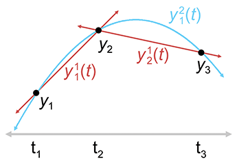
Consider the first quadratic curve, between
Since we have lots of curves at this point, we should invent some notation for them. We let
Take a look at the first quadratic curve
Now let's look at the math behind this. It's all linear interpolation. The easiest are the linear segments, which are defined by linear interpolation between the adjacent control points:
Linear interpolation between two control pointsThe quadratic curve is only slightly more complicated. We just linearly interpolate between the line segments:
Linear interpolation of lines yields a quadratic curveHopefully you can see the pattern—each curve is the result of linearly interpolating two curves of lesser degree. Aitken's algorithm can be summarized succinctly as a recurrence relation.
Aitken's algorithm works because, at each level both curves being blended already touch the
middle control points. The two outermost control points are touched by only one curve or the
other, but for those values of
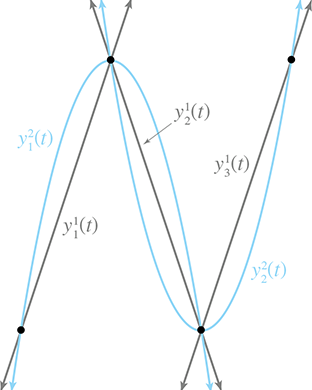
Now that we have the basic idea, let's apply it to our sideways S. Figure 13.4 shows Aitken's algorithm at work with our four data points. On the left, the three linear segments are blended to form two quadratic segments. On the right, the two quadratic curves are blending, yielding the final result that we've been seeking: a cubic spline that interpolates all four control points.
So we've successfully interpolated the four control points, and accomplished the goal set out at
the start of this section, right? Well, not exactly. Although our curve does pass through the
control points, it isn't really the curve we wanted. If we compare the curve on the right side of Figure 13.4 with the curve we set
out to create at the start of this section in Figure 13.2, we
see that the curve produced by Aitken's algorithm overshoots the
But don't despair! We've learned several important ideas that will be helpful when we discuss Bézier curves in Section 13.4 and splines in Section 13.6. In fact, we're going to beg your patience to allow us to extend the discussion on polynomial interpolation just a bit further. It's sort of like watching the movie Titanic; even though you know that the journey will end tragically, you still might find something useful along the way. We promise that the other techniques in this chapter will have practical as well as educational value.
By the way, you might have noticed that we didn't actually compute the polynomial
13.2.2Lagrange Basis Polynomials
Section 13.2.1 applied geometric intuition to the problem of polynomial interpolation and came up with Aitken's algorithm. Now we approach the subject from a more abstract mathematical point of view.
One mathematical approach to the interpolation problem comes from linear algebra.4 Each control point gives us one equation, and each coefficient gives us one unknown. This
system of equations can be put into an
Solving a matrix is a relatively time-consuming computational process, requiring
Let's ignore the
If we were able to create polynomials with the above properties, we would be able to use them as
basis polynomials. We would scale each basis polynomial
You might want to take a moment to convince yourself that this
polynomial actually interpolates the control points, meaning
Notice that the basis polynomials depend only on the knot vector (the
Of course, all of this would work only if we knew the basis polynomials, and finding
This trick works because at the knot
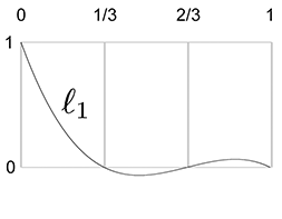
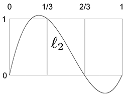
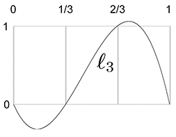
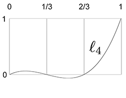
Let's apply this to our example S curve. Recall that it used the uniform knot vector
Figure 13.5 shows what these basis polynomials look like.
|
|
|
|
Now that we have the Lagrange basis polynomials for the knot vector, let's plug in the
Let's show these results graphically. First, we scale each basis polynomial by the corresponding coordinate value, as shown in Figure 13.6.
Finally, adding the scaled basis vectors together yields the
interpolating polynomial
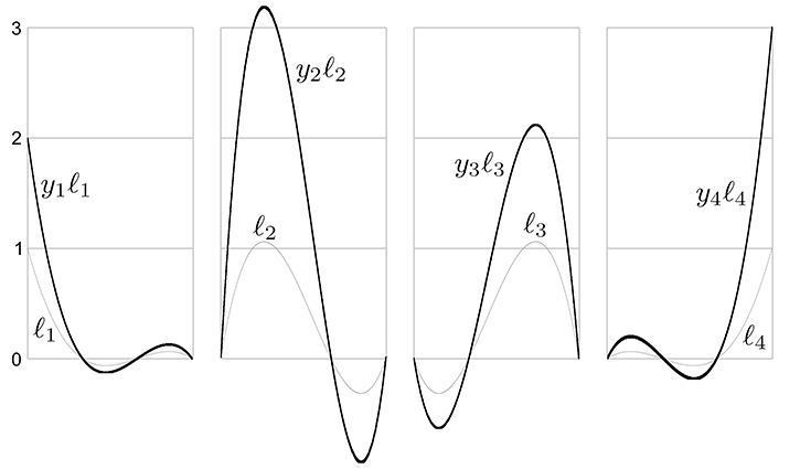
We use the word basis in basis polynomial to emphasize the fact that we can use these polynomials as building blocks to reconstruct absolutely any polynomial whatsoever, given the values of the polynomial at the knots. It's the same basic concept as a basis vector (see Section 3.3.3): any arbitrary vector can be described as a linear combination of the basis vectors. In our case, the space being spanned by the basis is not a geometric 3D space, but the vector space of all possible polynomials of a certain degree, and the scale values for each curve are the known values of the polynomial at the knots.
But there's an alternate way to understand the multiplication and summing that's going on. Instead of thinking about the polynomials as the building blocks and the control points as the scale factors, we can view each point on the curve as a result of taking a weighted average of the control points, where the basis polynomials provide the blending weights. So the control points are the building blocks and the basis polynomials provide the scale factors, although we prefer to be more specific and call these scale factors barycentric coordinates. We introduced barycentric coordinates in the context of triangles in Section 9.6.3, but the term refers to a general technique of describing some value as a weighted average of data points.
Notice that some values are negative or greater than 1 on certain intervals, which explains why
direct polynomial interpolation overshoots the control points. When all barycentric coordinates
are inside the
13.2.3Polynomial Interpolation Summary
We've approached polynomial interpolation from two perspectives. Aitken's algorithm is a
geometric approach based on repeated linear interpolation, and with it we can compute a point on
the curve for a given
Both methods yield the same curve when given the same data. Furthermore, this polynomial is
unique—no other polynomial of the same degree interpolates the data points. An informal
argument for why this is true goes like this: A polynomial of degree
For purposes of curve design, polynomial interpolation is not ideal, primarily because of our
inability to control the overshoot. The overshoot is guaranteed by the fact that the underlying
Lagrange basis polynomials are not restricted to the unit interval
Direct polynomial interpolation finds limited application in video games, but our study has introduced the themes of repeated linear interpolation and basis polynomials. We've also seen a bit of the beautiful duality between the two techniques.
13.3Hermite Curves
Polynomial interpolation tries to control the interior of the curve by threading the curve through specified knots. This doesn't work as well as we would like, because of the tendency to oscillate and overshoot, so let's try a different approach. We're still going to want to specify the endpoint positions, of course. But instead of specifying the interior positions to interpolate, let's control the shape of the curve through the tangents at the endpoints. A curve thus specified is said to be a Hermite curve or a curve in Hermite form, named in honor of Charles Hermite8 (1822–1901).
The Hermite form specifies a curve by listing its starting and ending positions and derivatives. A cubic curve has only four coefficients, which allows for the specification of just the first derivatives, the velocities at the endpoints. So describing a cubic curve in Hermite form boils down to the following four pieces of information:
-
The start position at
-
The first derivative (initial velocity) at
-
The end position at
-
The first derivative (final velocity) at
Let's call the desired start and end positions
Determining the monomial coefficients from the Hermite values is a relatively straightforward algebraic process of combining equations previously discussed in this chapter. The four Hermite values can be translated into the following system of equations:
Equations (13.9) and (13.12), which specify the endpoints, just repeat what we said in Section 13.1.5. Equations (13.10) and (13.11), which specify velocities, follow directly from the velocity equations for a cubic polynomial (Equation (13.5). The order in which these equations are listed is a convention used in other literature on curves, and the utility of this convention will become apparent later in this chapter.
Solving this system of equations results in a method to compute the monomial coefficients from the Hermite positions and derivatives:
Converting Hermite form to monomial formWe can also write these equations in the compact matrix notation introduced in
Section 13.1.2. Remember that when we put the coefficients as columns in a
matrix
where
The coefficient matrix
We can interpret the product
We emphasize that the adjectives “monomial,” “Hermite,” and “Bézier” refer to different ways of describing the same set of polynomial curves; they are not different sets of curves. We convert a curve from Hermite form to monomial form by using Equations (13.13)–(13.16), and from monomial form to Hermite form with Equations (13.9)–(13.12).
Let's take a closer look at the Hermite basis and hopefully gain some geometric intuition as to
why it works. Remember that we can interpret basis functions as functions of
Next, we name these basis functions (the rows of
Now, expanding the matrix multiplication makes it explicit that these functions serve as blending weights:
Interpreting the Hermite basis functions as blending weightsFigure 13.9 shows a graph of the Hermite basis functions.
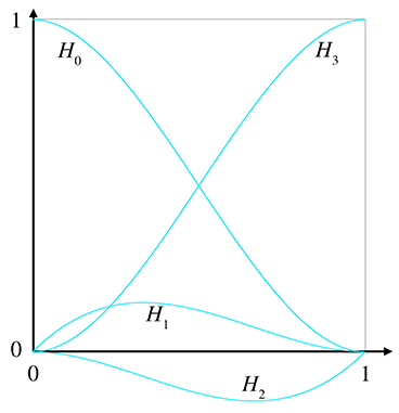
Now let's make a few observations. First, notice that
The curve
One final word about Hermite curves. Like the other forms for polynomial curves, it's possible to design a scheme for Hermite curves of higher degree, although the cubic polynomial is the most commonly used in computer graphics and animation. With the cubic spline, we specified the position (the “0th” derivative) and velocities (first derivatives) at the end points. A quintic (fifth-degree) Hermite curve happens when we also specify the accelerations (second derivatives).
13.4Bézier Curves
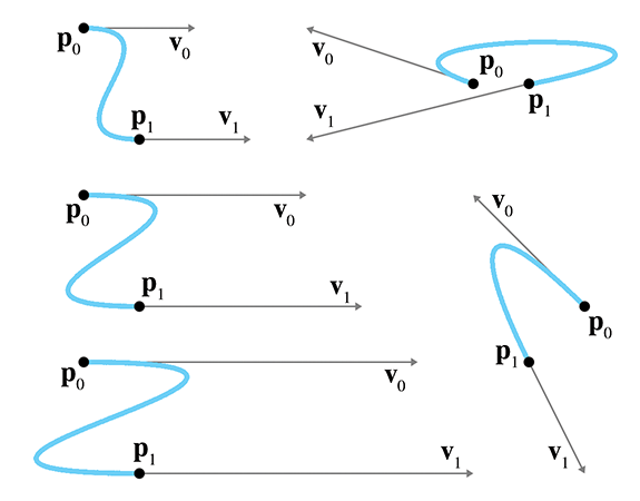
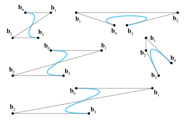
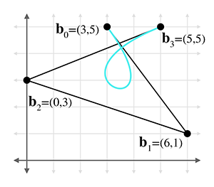
This chapter has so far discussed a number of ideas about curves that were enlightening, but it has yet to describe a fully practical way to design a curve. All of that will change in this section.10 Bézier curves were invented by Pierre Bézier (1910–1999), a French11 engineer, while he was working for the automaker Renault. Bézier curves have many desirable properties that make them well suited for curve design. Importantly, Bézier curves approximate rather than interpolate: although they do pass through the first and last control points, they only pass near the interior points. For this reason, the Bézier control points are called “control points” rather than “knots.” Some example cubic Bézier curves are shown in Figure 13.10.
Recall from Section 13.2 that the problem of polynomial interpolation had two solutions that produced the same result. Aitken's algorithm was a recursive construction technique that appealed to our geometric sensibilities, and a more abstract approach yielded the Lagrange basis polynomials. Bézier curves exhibit a similar duality. The counterpart of Aitken's algorithm for Bézier curves is the de Casteljau algorithm, a recursive geometric technique for constructing Bézier curves through repeated linear interpolation; this is the subject of Section 13.4.1. The analog to the Lagrange basis is the Bernstein basis, which is discussed in Section 13.4.2. After considering both sides of this coin, Section 13.4.3 investigates the derivatives12 of Bézier curves and reveals the relationship to Hermite form.
We've seen some beautiful cooperation between math and geometry in this book, but the convergence is particularly elegant for Bézier curves. It seems as if almost every important property of Bézier curves was independently discovered multiple times by researchers in different fields. Rogers' book [4] includes an interesting look at this story.
|
|
|
|
|
|
|
|
|
|
|
|
|
|
|
|
13.4.1The de Casteljau Algorithm
The de Casteljau algorithm defines a method for constructing Bézier curves through
repeated linear interpolation. It was created in 1959 by physicist and mathematician
Paul de Casteljau (1910–1999).13 We show how the algorithm works for the important cubic case as our
example. First, a bit of notation is necessary. A cubic curve is defined by four control points,
With that out of the way, let's consider a specific parameter value
It's helpful to write out all the
If we combine these recursive relationships with the basic linear interpolation formula, we obtain the de Casteljau recurrence relation.
Listing 13.1 illustrates how the de Casteljau algorithm could be implemented in C++
to evaluate a Bézier curve for a specific value of
Vector3 deCasteljau(
    int n,            // order of the curve, the number of points
    Vector3 points[], // array of points.  Overwritten, as
                      // the algorithm works in place
    float t           // parameter value we wish to evaluate
) {

    // Perform the conversion in place
    while (n > 1) {
        --n;

        // Perform the next round of interpolation, reducing the
        // degree of the curve by one.
        for (int i = 0 ; i < n ; ++i) {
            points[i] = points[i]*(1.0f-t) + points[i+1]*t;
        }
    }

    // Result is now in the first slot.
    return points[0];
}
This gives us a method for locating a point at any given
The linear case comes straight from the recurrence relation without any real work:
Applying one more level gives us a quadratic polynomial:
In other words, quadratic Bézier curves, which have three control points, can be expressed in monomial form as
Quadratic Bézier curve in monomial formBefore we do the last round of interpolation to get the cubic curve, let's take a closer look at
the quadratic expression in Equation (13.17). This conversion from
Bézier form to monomial basis can be written with fewer letters by using the matrix form
introduced earlier in this chapter. After putting the control points
As we saw in Section 13.3 with Hermite curves, the two different ways to group the
product
The other way to group the product
Back to repeated interpolation. One last round gives us the cubic polynomial:
One last iteration of de Casteljau iteration yields the cubic polynomial.\
Whew, expanding it all out like this is pretty exhausting!
Writing the last line again, but this time assuming the cubic level is the final level of recursion, we have
Cubic Bézier curve in monomial formJust to make sure you didn't miss it, Equation (13.19) tells us how to convert a cubic Bézier curve to monomial form. Since this is important, let's write it a bit more deliberately as
Cubic monomial coefficients from Bézier control points
We can now put this conversion into a matrix like we did with the quadratic case in
Equation (13.18). The cubic equation for a specific point on the
curve
We can also invert this process, meaning we can convert any polynomial curve from monomial form to Bézier form. Given any polynomial curve, the Bézier control points that describe the curve are uniquely determined:
Computing Bézier control points from monomial coefficientsAnd, of course, we can write this in matrix form:
Converting from monomial to Bézier form, in matrix notation13.4.2The Bernstein Basis
Section 13.4.1 ended with a bit of algebra to calculate the polynomial for a
curve from the Bézier control points. This polynomial was expressed in monomial form, meaning
the coefficients were for the powers of
Let's repeat the algebra exercise from Section 13.4.1, only this time we'll
be writing things in a slightly different way that will lead us to some observations. As we did
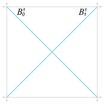
before, we start with the linear case (remember,
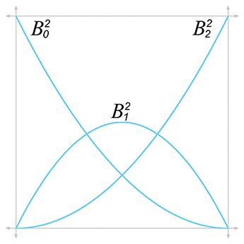
Next comes the quadratic:
And finally, we have the cubic case:
You might see a pattern emerging, but just to make it even more clear, let's show the curves up to degree 5 (we'll skip over the algebra; it's similar to what we did above):
Bézier curves of degree 1–5
Now the pattern is more clear. Each term has a constant
coefficient, a power of
The pattern for the constant coefficients is a bit more complicated. Please permit a brief, but hopefully interesting, detour into combinatorics. Let's write out the first eight levels in a triangular form to make the pattern a bit easier to see:
Pascal's triangle
With the exception of the 1s on the outer edge of the triangle, all other numbers are the sum of
the two numbers above it. You are looking at a very famous number pattern that has been studied
for centuries, known as the binomial coefficients because the
Binomial coefficients have a special notation. We can refer to the
For example,
Now let's look at the general formula for computing binomial coefficients. (We emphasize that
this formula is primarily for entertainment purposes, since our use of binomial coefficients in
this chapter on curves will be restricted to the first few lines of Pascal's triangle.) Remember
from Section 11.4.6 the
factorial operator, denoted
Using factorials, and defining
Binomial coefficients arise frequently in applications dealing with combinations and permutations, such as probability and analysis of algorithms. Because of their importance, and the amazingly large number of patterns that can be found in them, they have been the subject of quite a large amount of study. A very thorough discussion of binomial coefficients, especially regarding their use in computer algorithms, is presented by Knuth [2].
Back to curves. We've analyzed the pattern of the barycentric weights. Now let's rewrite a
Bézier curve, replacing each control point weight with a function
More generally, we can write a Bézier curve of degree
|
|
|
|
The function
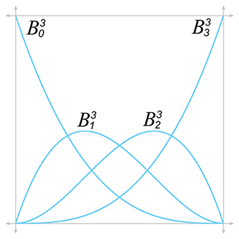
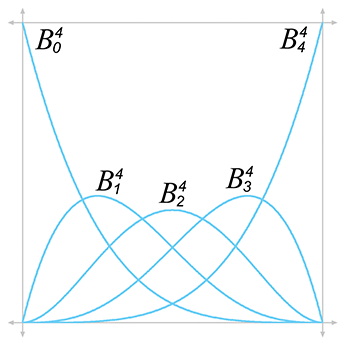
Figure 13.13 shows the graphs for the Bernstein polynomials up to the quartic case.
The properties of the Bernstein polynomials tell us a lot about how Bézier curves behave. Let's discuss a few properties in particular.
Sum to one. The Bernstein polynomials sum to unity for all values of
Convex hull property. The range of the Bernstein polynomials is
Endpoints interpolated. The first and last polynomials attain unity when we need
them to. Because
Global support. All the polynomials are nonzero on the open interval
Bézier control points have global support because the Bernstein polynomials are nonzero everywhere other than the endpoints. The practical result is that when any one control point is moved, the entire curve is affected. This is not a desirable property for curve design. Once we have a section of the curve that looks how we want, we would prefer that editing of some other distant control point not disturb the section that was shaped the way we liked it. This envious situation, known as local support, occurs when we move a particular control point and only the part of the curve near that control point is affected, for some definition of “near.”
Local support means that the basis function is nonzero only in some interval, and outside this interval it is zero. Unfortunately, such a basis function cannot be described as a polynomial, and thus no polynomial curve can achieve local control. However, local support is possible by piecing together small curves that fit together just right to form a spline, as Section 13.6 discusses.
One local maximum. Although each control point exercises influence over the entire
curve, each exerts the most influence at one particular point along the curve. Each
Bernstein polynomial
Thus, although every point on the interior of the curve is influenced to some degree by all the control points (because Bézier control points have global support), the nearest control point has the most influence.
13.4.3Bézier Derivatives and Their Relationship
to the Hermite Form
Let's take a look at the derivatives of a Bézier curve. Since we like to use the cubic curve as our example, we're talking about the velocity and acceleration of the curve. Remember that the velocity is related to the tangent (direction) of the curve, and the acceleration is related to its curvature.
Section 13.1.6 showed how to get the velocity function of a curve from the monomial coefficients:
Position and velocity of a cubic curveAnd Section 13.4.1 showed how to extract the monomial coefficients from a cubic Bézier curve:
Plugging these coefficients into the velocity formula (Equation (13.29)), we obtain a formula for the instantaneous velocity of a curve in terms of the Bézier control points:
First derivative (velocity) of a cubic Bézier curve
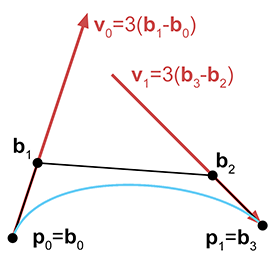
Now consider the velocity at the endpoints
This is interesting. Observe that
Another way to illustrate the role of the middle control points in a cubic Bézier curve is to
examine the relationship between the Bézier and Hermite forms. Remember that the cubic Hermite
form contains the initial position
Or, we can convert from Hermite to Bézier:
Converting cubic curve from Hermite form to Bézier formThus, Hermite and Bézier forms are very closely related, and it is very easy to convert between them. Their relationship is depicted graphically in Figure 13.14.
We've said that the first derivative at either endpoint is completely determined by the nearest
two Bézier control points. We can actually make a more general statement. The
At the endpoints, the acceleration is given by
Acceleration of a cubic Bézier curve at the endpointsAs expected, the acceleration at the start is completely determined by the first three control points, and the acceleration at the end is determined by the last three control points.
Let's define
The above discussion applies to Bézier curves of any degree. In general, the pattern is this:
if we move control point
13.5Subdivision
Beginning with Section 13.6, this chapter addresses the topic of joining together curves into a spline, which we can make as long and as complex as we want. Before we do that, this section considers the opposite problem: how to take a curve and chop it up into smaller pieces.
Why would we ever want to do this? There are a couple of reasons.
- Curve refinement. In the process of designing a curve interactively, we may find that we almost have the shape we want, but one curve can't quite give us the flexibility that we need. So we cut the curve into two pieces (forming a spline), which gives us greater flexibility.
-
Approximation techniques. Another reason to
subdivide a curve is that a piece of a curve is generally
simpler than the whole curve, where “simpler” means
“more like a straight line.” So we can cut it into a
sufficiently large number of pieces, and then do something with those
pieces as if they were straight line segments, such as render them
or raytrace them. In this way, we can approximate the result we
would get if we were able to render or raytrace the curve
analytically.
Strictly speaking, we don't need subdivision to do piecewise linear approximation—we already discussed one simple technique that evaluates the curve at fixed-size intervals and draws lines between those sample points. But subdivision allows us to choose the number of line segments adaptively by using fewer line segments on the straighter parts of the curve and more line segments on the curvier parts.
So that's the “why” of curve subdivision. Before we learn the “how,” let's be a bit more
precise about the “what.” Consider a parametric polynomial curve
The goal of subdivision is a mathematical description for
The following sections present two different methods for subdividing curves. Section 13.5.1 presents a straightforward algebraic approach in monomial form. Section 13.5.2 considers Bézier curve subdivision, which is geometrically based and lends itself towards rather elegant and efficient implementations.
Hermite form doesn't lend itself naturally to subdivision. If we wish to subdivide a Hermite form, we first convert the curve to another form (probably Bézier) and do the subdivision in that form.
13.5.1Subdividing Curves in Monomial Form
Extracting a segment from a curve in monomial form is a straightforward algebraic task. Remember
that monomial form is just an explicit polynomial on
With this in mind, we realize that the problem of subdivision can easily be viewed as a simple
problem of reparameterization. Rather than trying to muck directly with the monomial
coefficients, we perform some algebra on the parameter value. Let's introduce a local
parameter
where the function
You might want to verify that this does behave correctly at the endpoints.
Of course, all we have really accomplished is to define
However, the ensuing algebra gruntwork produces a messy result without revealing any insight. The main thing we wish to communicate here is that subdivision of a curve in monomial form is a simple matter of reparameterization, which can be accomplished algebraically. Furthermore, because we can convert between monomial forms and other forms, we now have a surefire method for subdividing any polynomial curve in any format.
But we need not be satisfied with this “brute force” approach; as it turns out, in Bézier\ form, we can do better.
13.5.2Subdividing Curves in Bézier Form
Subdivision of a Bézier curve can be done geometrically through a variant of the de Casteljau
algorithm. The full algorithm of extracting any subsection for arbitrary endpoint parameters
We begin by restricting ourselves to extracting only the “left side” of a curve. In other
words, we fix
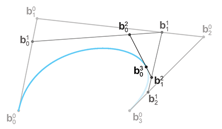
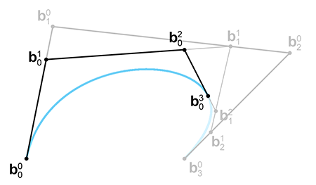
We have the endpoints—now for those tricky interior points. Surprisingly, if you look closely at Figure 13.16, you'll notice that we already constructed them! As it turns out, each round of de Casteljau interpolation produces one of our Bézier control points. Figure 13.17 makes this clearer, showing the selected Bézier points and the control polygon.
Why does this work? Recall the relationship between the Bézier form and the Hermite form from
Section 13.4.3. The first interior control point
Let's summarize our findings. To extract the left half of a curve,
There is one important special case of Bézier subdivision that we can do armed only with what
we know so far: subdividing a curve “in half” at
The general case is obtained through blossoming, which is a general term referring to a
number of techniques involving repeated de Casteljau steps taken with different interpolation
fractions. To determine each control point, we take three de Casteljau steps (for a cubic curve,
at least). For each control point
13.6Splines
So far we have been focusing on cubic curves, and for good reason; they are the most commonly used type of curves in 3D. Such curves inherently have four degrees of freedom, whether we are using Bézier curves with four control points, monomial curves with four coefficients, or Hermite curves with two ending points plus two derivatives. Because there are only four degrees of freedom, the set of curves that can be represented by using only the techniques of cubic curves is sharply limited.
Additional freedom is obtained by joining smaller curves together in a spline, which is
the subject of the remainder of this chapter. Before we discuss splines, let's pause for a
moment to discuss one potential alternative: using a higher degree polynomial. Obviously any
degree
In Bézier form, degree elevation adds a new control point and, as you might have guessed, the
positions of the new control points can be constructed geometrically by using linear
interpolation. Given a curve of degree
(Note that the computation of
For Hermite curves, we usually are interested only in odd values for
A higher degree polynomial has the ability to describe a curve with more “wiggles,” but, unfortunately, in general it suffers from several shortcomings:
- The curve has global support. Each control point exerts some nonzero weight on every point along the curve, with the exception of the endpoints.
- The curve has extraneous “wiggles” that sometimes show up in places we don't want, oscillating back and forth between the control points. This is known as the Runge17 phenomenon.
- Somewhat related to the extra wiggles is the fact that higher degree curves are very sensitive. Due to the curve's global support, a change to any one of the control points will result in a change over the entire curve; due to the high sensitivity, this response can be very large.
- Having ruled out polynomial interpolation as a viable curve design tool, we cannot directly specify a point that we want the curve to interpolate, other than the endpoints.
The basic problem is that we are asking too much from a single polynomial. Splines do not have these shortcomings.
Here's what's in store. First, to facilitate the discussion, we must expand our notation and introduce a level of indirection between the local and global parameterization, which we do in Sections 13.6.1 and 13.6.2. Then, in Section 13.7, we talk about Hermite and Bézier splines, which are used in many software packages, such as Adobe Photoshop and Autodesk 3DS Max. From there, our focus naturally gravitates towards deciding what to do at the “seams.” The first hurdle is to define the criteria that must be met so that the curve is smooth at these junction points. Such continuity conditions are the subject of Section 13.8. Once we understand these issues, we will have finally reached our goal set at the start of this chapter, a spline system that provides an intuitive means to define a curved shape.
Having developed a flexible design tool where the user can specify the position and tangent at each control point, Section 13.9 then investigates methods by which the designer need specify only the positions of the control points, and the tangents are computed automatically based on a set of intuitive user controls.
13.6.1Rules of the Game
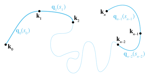
Our spline is composed of
We use two different notations to refer to the entire spline. One way is to just drop the
subscripts from the notation above, so the function
The composite function
Note that, given a particular value for
If we are not concerned with the timing of our curve, then this notation may be all we need.
However, when defining an animation path, we usually need a level of indirection. We introduce
the notation
In general, we can define
With the above notation established, the basic game plan for evaluating
-
Map the time value
-
Extract the integer portion of
-
Evaluate the curve segment
Of course, if we don't care about the timing of the spline (perhaps we only care about its
shape), then we have no need of the first step, and we can just use the trivial mapping of
With the assumption for now that
13.6.2Knots
Think about the juncture between two segments. For the curve to be continuous, clearly the
ending point of one segment must be coincident with the starting point of the next segment.
(Section 13.8 addresses additional desirable criteria.) These shared control points
that are interpolated by the spline are called the knots of the spline. The knot at index
We assume that the segments are connected at the knots. In other words,
Note that
In animation contexts, the knots are sometimes called keys. This is a reference to the old-school animation methods where a master animator would create the key frames, or frames where the characters reached important poses. The in-between frames would be filled in by a less experienced (and less expensive) apprentice. In computer animation, a key can be any position, orientation, or other piece of data whose value at a particular time is specified by a human animator (or any other source). The role of the apprentice to “fill in the missing frames” is played by the animation program, using interpolation methods such as the ones being discussed in this chapter. As we've noted before, most of the early research on splines was aimed at defining static shapes, not animated trajectories, and so the term “knot” is more prevalent.
13.7Hermite and Bézier Splines
A spline is made by patching together curve segments so that they fit together smoothly. What sorts of curve segments? For reasons that will soon become apparent, it is most convenient for us to use the Hermite representation for the individual segments. When we say convenient “for us,” we mean the people writing the code for an animation system or carrying out the mathematical discussion in the following sections. When it comes to depicting or manipulating splines graphically, the Bézier form is typically preferred. Of course, the Hermite and Bézier forms are closely related, and it is easy to convert between the two forms. If you don't remember this relationship, we review it in just a moment.
Remember that a Hermite curve segment is defined by its starting and ending positions and
velocities. When we were focused on a single segment, we denoted the positions by
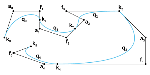
Figure 13.19 shows a spline with five Hermite segments. All of the knots, segments, and tangents are labeled according to the notation just described.
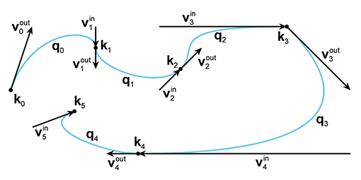
Be warned that the tangents in Figure 13.19—and all the figures of Hermite curves in this chapter—are drawn at one-third scale. Officially we'd like to tell you that this was done so that the diagrams would be smaller and this book would consume less of the Earth's natural resources. A more accurate reason is that we draw the tangents at one-third length so the tangents will be the same as the edges of the Bézier control polygon. Matching the Bézier control polygon has some educational benefits, but, more importantly, it facilitates laziness on the part of the authors: the tools we used to create the curves in the diagrams are based on Bézier splines.
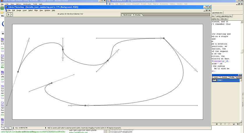
The splines in the diagrams in this book were created in Adobe Photoshop by making a path and then “stroking” the path. The arrows for the tangent vectors were drawn by putting one end at a knot and the other end at the “handle” used to control the shape of the curve, which is essentially the same as the Bézier control point. (Photoshop calls the knots the “anchor points” and refers to the interior Bézier control points that are not interpolated as “control points.”)
For example, Figure 13.20 is a screen capture taken while one author was hard at work creating Figure 13.19. (The opacity of the actual figure has been decreased to make it easier to see the Photoshop controls.)
While we're on the subject of Bézier curves, let's take this opportunity to introduce the
notation we use for Bézier splines. When we were dealing with only a single Bézier segment,
we referred to the
The important relationship between Hermite and Bézier forms was introduced in Section 13.4.3. Let's restate it here in the newly-introduced spline notation:
Converting between Bézier and Hermite forms13.8Continuity
For a few sections now we've been promising to tell you how you can piece together segments into
a spline such that they fit together smoothly. All this lead-up may have given the impression
that it's a mysterious secret. But if you take a closer look at
Figure 13.19, you'll see that the criterion is relatively obvious: if the
incoming and outgoing velocity vectors are equal at a knot, as they are at
Consider the curve near
Speaking of smooth animations, we just said that the curve is smooth at
Finally, consider a knot for which the incoming and outgoing velocities are both zero. In this case, even though the tangents are continuous, most people would agree that the shape is not smooth at this knot. What about the motion? Is the motion smooth when we come to a complete stop and then accelerate away in a potentially different direction? That will depend on your needs.
It looks like the answer to the question “Is it smooth?” is a bit fuzzy. This is a mathematics book, and it's really bad form to be putting quotation marks around vague words such as “smooth.” We really need some more precise terminology. In the context of curves, the most important smoothness criteria are parametric continuity and the closely related geometric continuity. Let's look at each of these in turn, starting with parametric continuity, which is easier to define mathematically.
13.8.1Parametric Continuity
A curve is said to have
Higher numbers for
Any individual polynomial curve segment by itself has
One last comment regarding higher derivatives. When we say that a curve is
Now that we've discussed parametric continuity informally, let's define the criteria mathematically for Hermite and Bézier curves. To do so, we make use of some observations concerning the derivatives of Bézier curves from Section 13.4.3; our findings from that section are summarized here.
-
The
- The velocity at an endpoint is proportional to the vector between the endpoint and the adjacent control point (Equations (13.30) and (13.31)).
- The acceleration at an endpoint is proportional to the difference of the delta vectors along the nearest two segments of the control polygon (Equations (13.36) and (13.37)).
Let's start with
and with just a little effort we can also express it in Bézier form as
With a quick application of algebra, we see that geometrically this means that the knot is at the
midpoint of the line between
Most curve design tools will automatically enforce this rule for you. For example, when you move
a control point in Photoshop, it automatically moves the opposing control point like a
seesaw, and if you pull the control point away from the anchor point (the knot), the opposing
control point will mirror your movements to maintain the
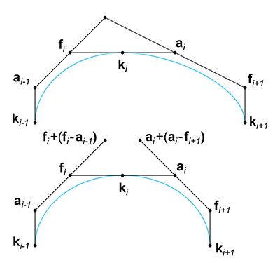
Now let's look at
The geometric interpretation of this is as follows: Take the two Bézier control polygon
segments that are not direct neighbors of the knot, but one segment away, and “double” them. If
they meet at a common point, the curve is
13.8.2Geometric Continuity
Geometric continuity is a broader criterion of continuity. Different authors use
different definitions for geometric continuity, but a very general one is that a curve has
In Figure 13.19 the curve is not
Higher-order geometric continuity extends this idea, although it is a bit more difficult to
visualize. We say that a curve is
13.8.3How Smooth Can a Curve Be?
We end our discussion on continuity by asking an important question: what's the highest level of
continuity we can expect from a polynomial spline? We said earlier that any particular curve
segment has
Consider two adjacent cubic Bézier segments. Let's fix the first segment and consider what
happens to the second segment as we demand higher and higher levels of continuity at the knot.
When we demand
What about
Continuing this pattern, we see that for a Bézier segment to match
The bottom line is that, practically speaking, a polynomial curve of degree
13.9Automatic Tangent Control
At the start of this chapter, we began our investigation into curves with the plan of defining a curve just by listing points that we wanted the curve to pass through. We tried basic polynomial interpolation in Section 13.2, but found that it didn't give us what we wanted. We then developed the Bézier forms, which require the user to specify two endpoints, which are interpolated, and two (in the case of a cubic Bézier) interior control points, which are not interpolated but instead define the derivatives at the endpoints. So far in this chapter, we've learned how to piece together those Bézier segments in a smooth spline.
This section investigates various methods whereby a spline can be determined by just the knots, without the need for the user to specify any additional criteria. This is useful to generate a curve that looks “natural” and passes through some points, or any other time we wish to smoothly interpolate some data points.
For the moment, let's ignore the first and last knots and focus our attention on the interior
knots. The problem at hand is to compute an appropriate
The following sections discuss a family of techniques that can be used to pick tangents that result in “good” interpolating splines. First, Section 13.9.1 discuss the Catmull-Rom spline, which is a simple and straightforward technique. Then Section 13.9.2 considers TCB splines, a generalization of the Catmull-Rom form and a hybrid that exposes additional “sliders” to the user to adjust the shape of the curve in a (hopefully) more intuitive manner without resorting to direct geometric specification of the tangents. Finally, Section 13.9.3 lists a few options for dealing with the endpoints.
When reading the following sections, keep in mind that all of these splines are still Hermite splines. We are just introducing various techniques for autocalculating the tangents. Once the tangents have been determined, the spline is no different than any other Hermite spline.
13.9.1Catmull-Rom Splines
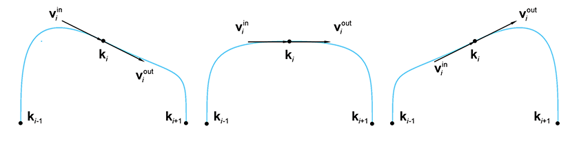
Looking at Figure 13.23, it seems obvious which of the three choices
of tangents is the most natural: the one in the middle. Why is this? The vector from the
previous knot
But how long should the tangents be? Perhaps we should again use the vector between the previous
and next knots as our guide. It seems as though the farther apart our neighbors are, the larger
the curve, and so making our tangents be a constant multiple of this vector would be a good idea.
In other words, we would set
One way would be just to experiment and find a nice round number that seems to give results that
are aesthetically pleasing. The constant
Although
First, let's give a formal definition and name to this technique. A spline with the tangents derived according to the relation
Tangent computation for the Catmull-Rom spline and its Bézier control polygonis known as a Catmull-Rom spline. The name comes from the two people who invented it, one of whom is Edwin Catmull (1945–). He later went on to become the president of Walt Disney Animation Studios and Pixar Animation Studios.
The other thing we'd like to discuss is an alternative way to derive Equation (13.39). Just a bit of algebraic manipulation yields
Catmull-Rom spline as average of adjacent delta vectorsThe geometric interpretation of the last line states that to compute a tangent at a knot, we take the two neighboring difference vectors of the control polygon and average them.
13.9.2TCB Splines
Section 13.9.1 showed that the tangent at a knot can be computed by multiplying the
vectors of the adjacent edges of the control polygon by an appropriate constant, which we called
Kochanek and Bartels [3] designed the equations so that if we turn all three
dials to zero, we get the standard Catmull-Rom curve. The typical useful range for all of the
parameters is
The tension setting is related to the
Note that
We incorporate tension into the Catmul-Rom tangent formula as follows:
Catmull-Rom formula extended to allow tension adjustmentsNext let's turn to the continuity setting, which can be used to break the smoothness of
the curve and force a corner at the knot. The value of zero will result in equal tangent (no
matter what values for tension and bias are used), thus ensuring
One important observation to note is that setting
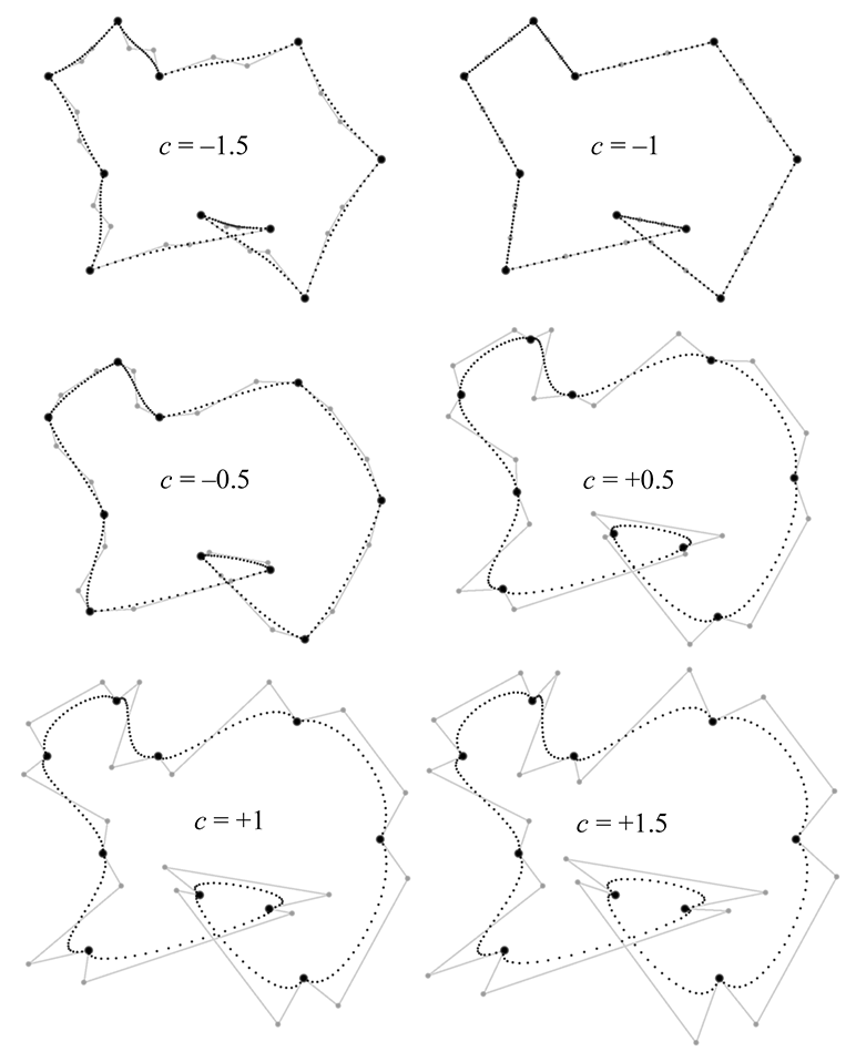
The math behind TCB continuity is written as
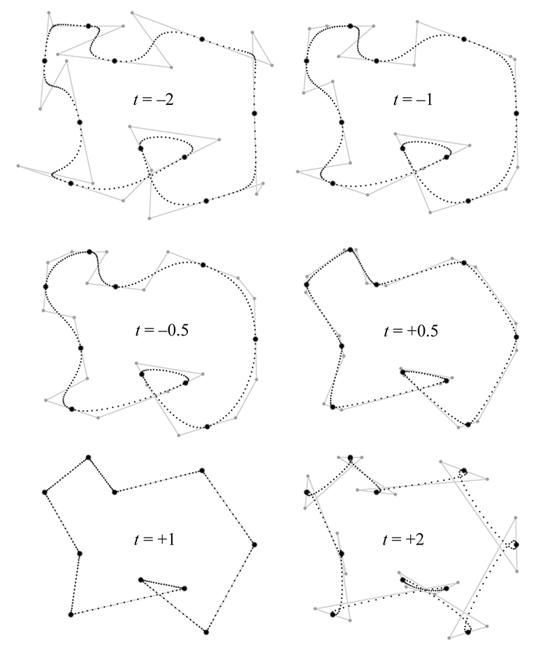
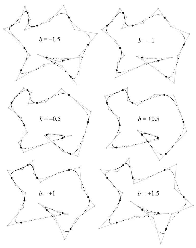
Catmull-Rom formula extended to allow continuity adjustmentsFinally, the bias argument can be used to turn the tangents towards one or the other adjacent knots, rather than being parallel to the line between the adjacent knots, as the Catmull-Rom curve does. Consider a sequence of three knots. A negative bias causes the curve to “anticipate” the third knot, turning the curve in the direction of the third knot a bit before the middle knot is reached. In contrast, a positive bias value causes the curve to wait to make the turn towards the third knot, causing some “overshoot” through the middle knot. Figure 13.27 shows our example spline with several different bias values.
The bias value works by scaling the relative weights that the two control polygon edges have on the resultant tangent:
Catmull-Rom formula extended to allow bias adjustmentsThe equations presented thus far have isolated each setting to make it easier to understand the math behind each one. Now let's put all three settings together:
One last note. The examples in this section used the same values at each knot in the spline, but that need not be the case. The TCB values are often adjusted on a per-knot basis.
13.9.3Endpoint Conditions
The Catmull-Rom methods rely on the previous and next knots to compute the tangent at a given knot. What should we do at an endpoint when there is no “previous” or “next” knot? Several solutions to this problem have been proposed.
One obvious answer would be to just throw our hands in the air and set the tangent to zero at an endpoint. While this seems like surrendering before the first shot is fired, it actually can be a good choice if the spline is to be used for animation, since it's often natural to want the object being animated to start and end “at rest.”
Another idea is to create extra knots
One final method is to fit the first (or last) three knots to a quadratic, and use the endpoint tangent of this curve. The curve fitting is an example of polynomial interpolation and can thus be done by using the techniques from earlier in this chapter, such as Aitken's algorithm.
Exercises
-
Compute the Lagrange basis polynomials for the knot
sequence
-
The motion of a projectile
(see Section 11.6) can
be described by the quadratic function
where
Imagine you want to animate the path of a projectile—say, a herring sandwich. Assume you are working in our standard 3D coordinate space (see Section 1.3.4) and the object is launched from the origin, reaches a maximum at -
Consider the Bézier curve in the figure below.
- (a)Use de Casteljau to determine the position on the curve at
- (b)Convert the curve to Hermite form.
- (c)Convert the curve to monomial form.
-
(d)Check your work on part (a) by substituting
- (e)What is the velocity polynomial function
- (f)What is the velocity at
- (a)Use de Casteljau to determine the position on the curve at
-
Prove that the quadratic Bernstein basis polynomials sum to 1 for any value of
-
Where should we put the Bézier control points to get a
“constant curve” where
- Where should we put the Bézier control points to get a linear “curve,” which is a straight line segment with constant velocity?
- Where should we put the Bézier control points to get a straight line shape, but this time the velocity of the curve follows the smoothstep pattern: it starts at zero, accelerates to a maximum velocity at the middle, and then decelerates to end with zero velocity?
-
Describe the motion of a particle that moves along the
Bézier curve where
- Consider the projectile herring sandwich from Exercise 2. Assume you need to animate this sandwich, and the only tools available to you are cubic Bézier\ curves. Where should you put the four Bézier control points to get physically realistic motion, which is quadratic? Don't worry about the total duration the sandwich is airborne; consider only the shape of the trajectory.
-
To plot the shape of the parabola
in Figure 12.8
,
the authors tabulated a list of
-
Returning to the curve in Exercise 3:
- (a)Compute the Bézier control points for the segment of the curve from 0.2 to 0.5.
-
(b)Split this curve into two halves at
- (c)Perform degree elevation on this curve to the quartic case. What are the five control points?
- This is not intended as a comment on a certain Australian children's musical group, but may be misinterpreted as such.
- Aitken's Al Gore rhythm, if you will.
- Don't try this excuse with your professor, but it's been known to work in job interviews.
- We're talking about real linear algebra, not the geometry-focused subset of it we study in this book.
- This type of matrix, in which each row or column is a geometric series of the powers of some term, is known as a Vandermonde matrix, after the French mathematician Alexandre-Théophile Vandermonde (1735–1796).
- Although they are named for Joseph Louis Lagrange (1736–1813), Lagrange basis polynomials were discovered in 1779 by Edward Waring (1736–1798). It may be interesting to some readers that Lagrange is Ian Parberry's PhD adviser's PhD adviser's,…, PhD adviser back 10 iterations.
- It's important to pronounce the name of this French mathematician “luh-GRAWNGE”. Otherwise, people might think you are talking about the small Texas town of La Grange (pronounced “luh-GRAYNGE”). To the authors' knowledge, La Grange, Texas is not the namesake of any basis polynomials, although ZZ Top did name a song after the town in honor of a nearby brothel.
- He's another French guy, and his mother probably pronounced his name “air-MEET.” But many English speakers, even some we know with PhDs, pronounce it “HUR-mite,” so you can probably do the same.
- If you're one of those purists who objects to the idea of “blending” points with vectors (see Section 2.4), don't worry. It's possible to interpret the equations such that the offensive comingling does not occur.
- Well, just some of that is going to change—we hope your reading will still be enlightening. You know what we mean.
- See, we told you a lot of these guys were French! By the way, it's pronounced “BEZ-ee-ay.”
- “Rate of exchange,” if you will pardon the pun.
- Yep, he's French, too, and that means you'd better pronounce his name correctly: “duh CAS-tul-jho.” He worked for Renault's rival, Citroen.
- Yes, he was French, too. He appears in Ian Parberry's PhD adviser tree somewhat off to the left back 16 generations.
- In addition to his triangle, Pascal has an SI unit of pressure, a law, a programming language, and a wager named after him, although the latter two are no longer in serious use.
- Russian, not French.
- Pronounced “RUN-guh.”
-
Note that by using knot-centric
notation and assigning different letters to the control points (based on handy mnemonic memory
aids!), we are locking in the degree of the segments to cubic. In other sources you'll find
notation such as
- Oops, there are the quotation marks that we just said were bad form in a math book!
- The most important for us is that TCB is easier to pronounce than koh-CHAN-ick.